Agenda
- Introduction
Scientific Visualization
Scientific Visualization Pipeline
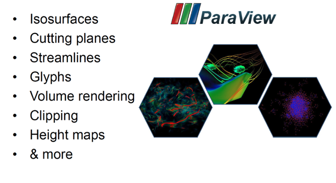
Common Sci-Vis Techniques
- Introduction to ParaView
- Hands-on Exercises
Scientific Visualization
Scientific Visualization Pipeline
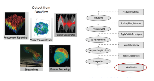
Common Sci-Vis Techniques
Overview
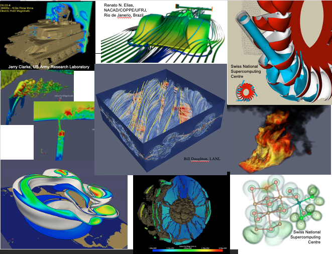
Scientific visualization primarily concerned with the visualization of three dimensional phenomena like architectural, meteorological, medical, biological, etc.
Its emphasis is on realistic renderings of volumes, surfaces, illumination sources, and so forth, perhaps with dynamic (time) component.
The benefits include improved communication and efficiency as well as better management and decision making.
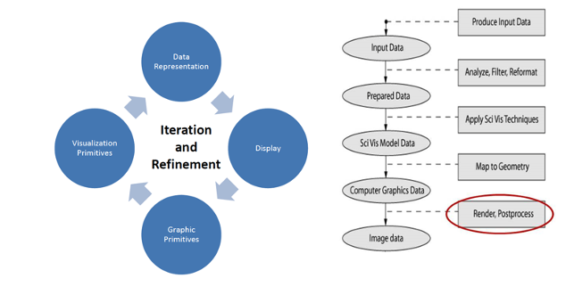
Visualization Pipeline
Basics of Visualization
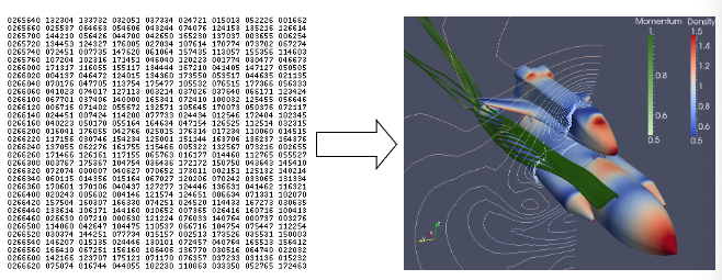
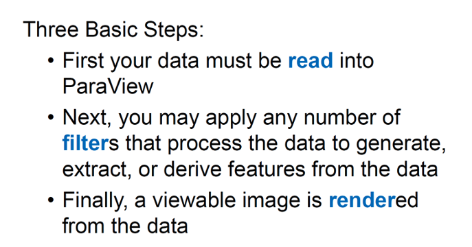
The fundamental concept of visualization involves the transformation of raw data into meaningful visual representations, which serve the purpose of providing valuable insights.
Scientific Visualization Pipeline:
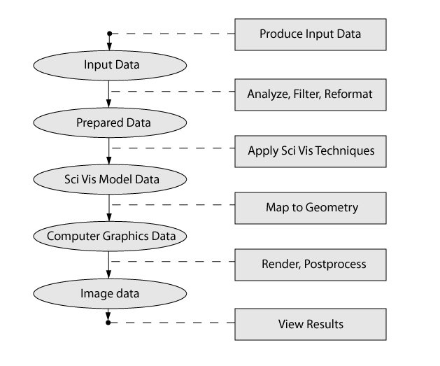
Scientific Visualization Pipeline:
Adapted from BU Tech
-
Produce Data
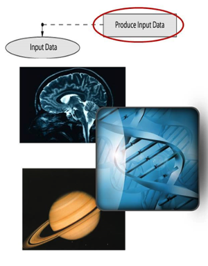
1. Simulated Data
2. Images
3. Numerical
4. Some measured value
5. Observed phenomena -
Analyze, Filter, Reformat
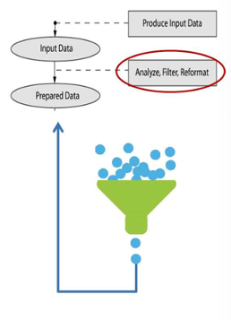
Cleaning up the data
1. Removing noise
2. Replacing missing values
3. Clamping values to be within a specific range of interest
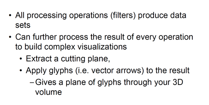
Performing operations to yield more useful data -
Apply SciVis Techniques
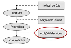
Converts raw information into something more understandable.
Visually extracting meaning from a scinetific dataset using various techniques.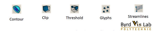
-
Map to Geometry
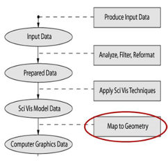
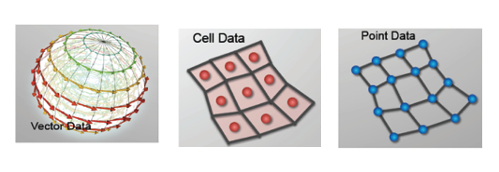
1. Scalars, vectors, tensors
2. 1D, 2D, 3D
3. Mesh
-
Render, Post Process
-
Results
Visualization Toolkit [VTK]
- Open source, multiplatform
- Supports distributed computation models
- Extensible, modular architecture
- Available for 3D computer graphics, image processing and visualization
- Collection of C++ libraries
- Leveraged by many applications
- Divided into logical areas
- Filtering
- Information Visualization
- Volume Rendering
- Cross platform, using OpenGL
- Wrapped in Python, Tool Command Language (TCL) and Java
- Filtering
- Information Visualization
- Volume Rendering
Software: ParaView
Paraview is a powerful software tool widely used in scientific visualization to explore and analyze complex data sets. Designed for researchers and scientists, Paraview facilitates the creation of interactive and
immersive visualizations that provide deeper insights into scientific phenomena. With its versatile range of visualization techniques and advanced rendering capabilities, Paraview enables the representation
of diverse data types, including numerical simulations, computational models, and experimental results. Its intuitive interface and extensive customization options make it a valuable tool for understanding and
communicating scientific data effectively.
It is an end-user application with support for:
1. Parallel Data Archiving
2. Parallel Reading
3. Parallel Processing
4. Parallel Rendering
5. Single node, Client-Server, MPI Cluster Rendering
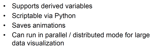
More Paraview features:
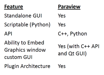
Paraview Summary:
Basics of Paraview
-
Data Ranges
-
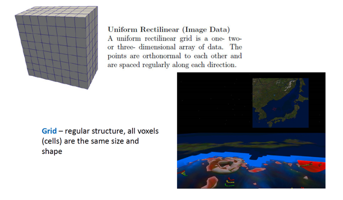
Supported Data Types
It is an end-user application with support for:
1. Point Data
2. Polygonal data
3. Images
4. Multi-block
5. Adaptive Mesh Refinement
6. Time series support -
Supported Visualization Algorithms
-
Special Features
-
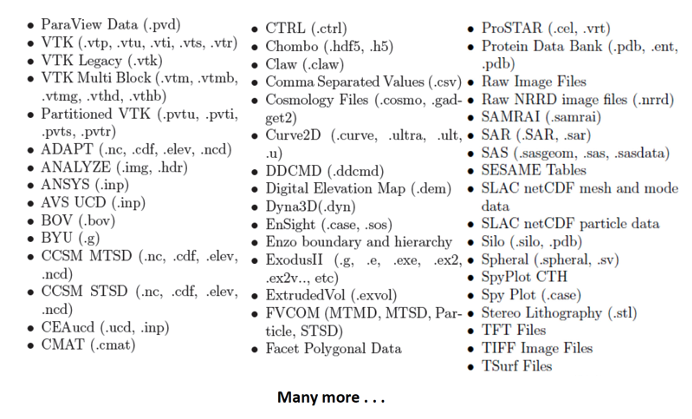
Supported File Formats
-
Visualization Pipeline
-
Visualizing Data using Paraview
Tutorial
ParaView is a powerful scientific visualization software that empowers researchers and scientists to explore, analyze, and communicate complex data sets. By providing an intuitive and versatile platform, Paraview
enables the transformation of scientific data into visually compelling representations, facilitating the understanding of intricate patterns and structures. With its extensive range of visualization techniques
and interactive features, Paraview offers an essential tool for investigating scientific phenomena, uncovering insights, and conveying findings effectively in various fields such as physics, engineering,
medicine, and environmental sciences.
We will be going through the steps to create visualizations using Paraview.
Step 0: Understanding the Interface
- User Interface
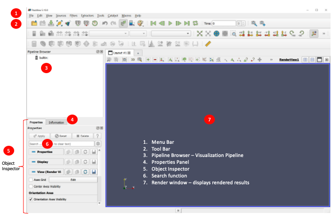
Figure 1: User Interface
- Simple Camera Manipulations
- Drag left, middle, right buttons for rotate, pan and zoom.
- Also use Shift, Ctrl, Alt modifiers
- Also try holding down x, y, z
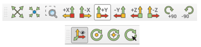
Figure 2: Camera Manipulations
- Getting Back Graphical User Interface(GUI) Components
- Menu Bar
- View -> Toolbars
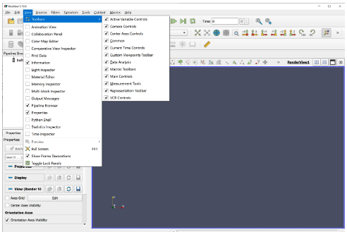
Figure 3: GUI Interface
- Help Menu
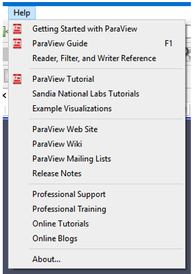
Figure 4: Help Menu
- Undo/Redo
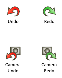
Figure 5: Undo/Redo
- Copy/Paste/Reset/Save Parameters
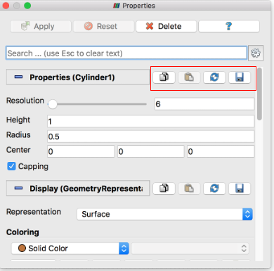
Figure 6: Copy/Paste/Reset/Save Parameters
- Pipeline Object Control
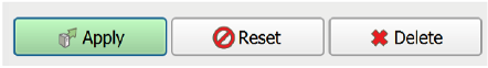
Figure 7: Pipeline Object Control
- Using Auto Apply
- Click Auto Apply.

- Change the Resolution parameter (or any other parameter).
- Note that the visualization automatically updates without having to hit Apply.
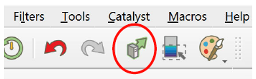
Figure 8: Auto Apply
- Drag left, middle, right buttons for rotate, pan and zoom.
- Also use Shift, Ctrl, Alt modifiers
- Also try holding down x, y, z
- Menu Bar
- View -> Toolbars
- Click Auto Apply.
- Change the Resolution parameter (or any other parameter).
- Note that the visualization automatically updates without having to hit Apply.
Step 1: Creating a Cylinder Source
- Go to the Sources menu.
- Select Geometric Shapes.
- Select Cylinder.
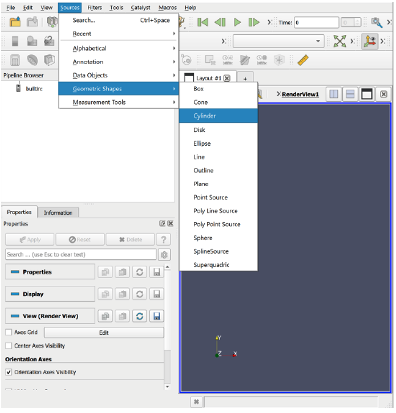
Figure 9: Sources
- A Cylinder1 object should appear in the pipeline browser
- If the cylinder does not automatically appear in the 3D viewer click the Apply Button (on the Properties Tab)
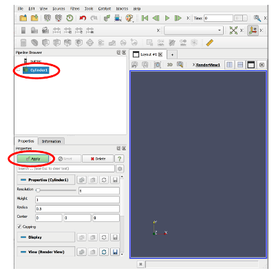
Figure 10: Creating Cylinder
- Explore the resolution feature
- Adjust the Resolution slider
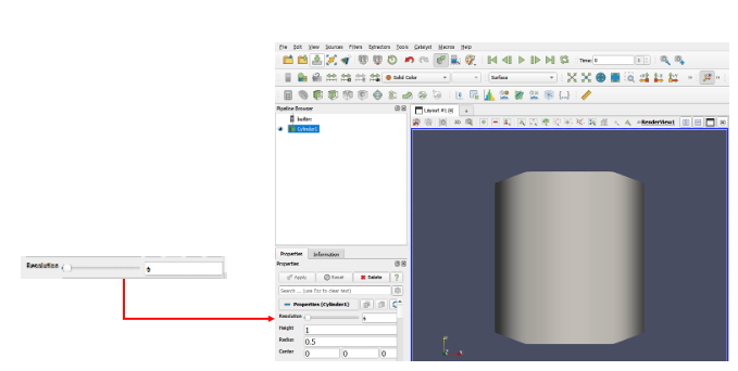
Figure 11: Resolution slider
- Explore the resoulution feature by adjusting the Resolution slider or type in a value.
- Click the Apply button to accept changes.
- Display Properties
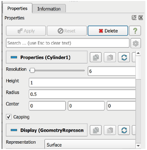
Figure 12: Display Properties
- Change Render Properties
- Scroll down to the Display (Geometry Representation) section
- Click the Edit button. This button is replicated in the tool bar
- Select a new color for the cylinder.
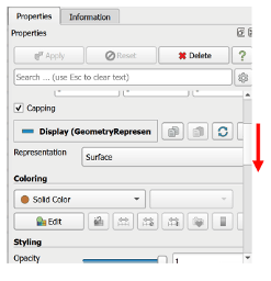
Figure 13: Edit Color
- Render View Options
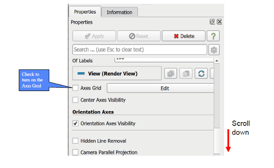
Figure 14: Render View Options
- Resulting Cylinder
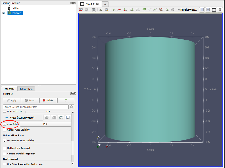
Figure 15: Resulting Cylinder
- Changing the Color Palette
- Make sure the orientation axes are visible in the lower left corner.
- Click the color palette button and change the colors.

- Try several color palettes or edit the current color palatte.
- Edit Color Palette
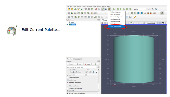
Figure 16: Edit Color Palette
- Choose Color Palette
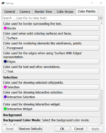
Figure 17: Choose Color Palette
- Advanced Properties
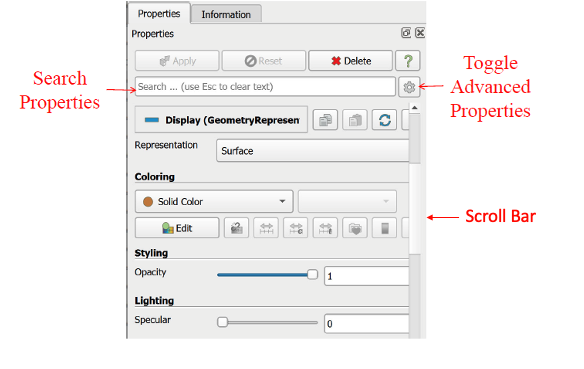
Figure 18: Advanced Properties
- Searching Properties
- Type “specular” in the properties search box
- Change Specular value to 1 (makes the cylinder shiny)
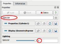
Figure 19: Specular
- Other interesting properties incluse Axes Grids and Opacity amongst others.
- Scroll down to the Display (Geometry Representation) section
- Click the Edit button. This button is replicated in the tool bar
- Select a new color for the cylinder.
- Make sure the orientation axes are visible in the lower left corner.
- Click the color palette button and change the colors.
- Try several color palettes or edit the current color palatte.
- Type “specular” in the properties search box
- Change Specular value to 1 (makes the cylinder shiny)
- Other interesting properties incluse Axes Grids and Opacity amongst others.
Step 2: Let's start working with Training data.
- Click on the button on the banner saying “Edit” and then "Reset".
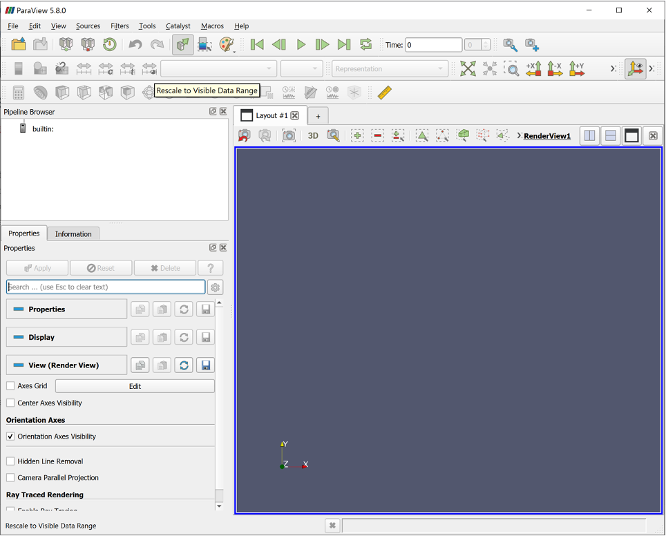
Figure 20: Paraview Interface
- Click on the button on the banner saying “File” and then "Open" after locating the file 'headsq.vti'
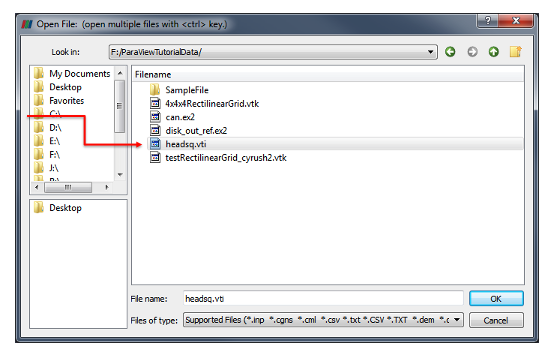
Figure 21: Open File
- New Object in Pipeline Browser
- Click Apply to update the viewer window if necessary.
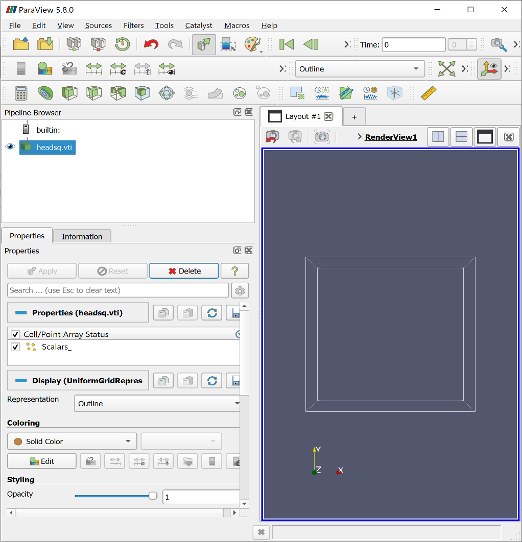
Figure 22: Viewer
- You should see a bounding box in the 3D viewer window
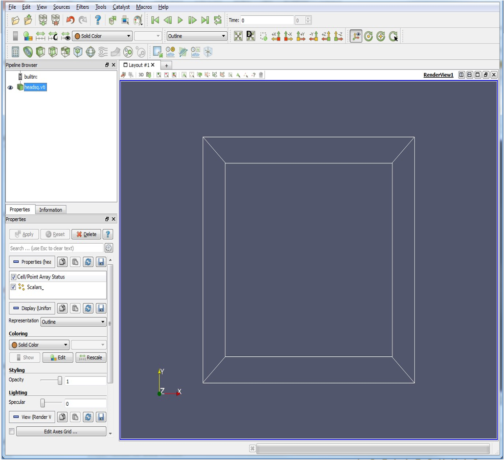
Figure 23: Viewer with bounding box
- New Object in Pipeline Browser
- Click Apply to update the viewer window if necessary.
- You should see a bounding box in the 3D viewer window
Step 3:: Creating an Isosurface
- On the upper ribbon, you will find a tab called "Filters". Click on Common and then Contour
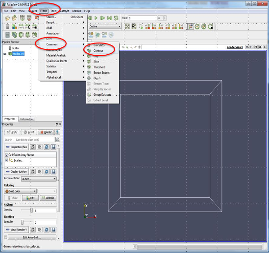
Figure 24: Isosurface Selections
- A new object appeared in the pipeline browser (Contour 1)
- Contour – Extracts the points, curves, or surfaces where a scalar field is equal to a user-defined value.
The surface is often also called an isosurface.
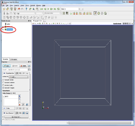
Figure 25: Isosurface
- Value Range for the data set is now visible
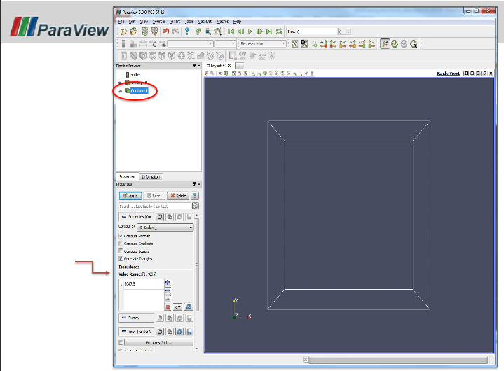
Figure 26: Value Ranges
- Value Range for the data set is [ 0, 4095 ]
- Only one value is showing: 2047.5
- Click Apply to see what points, curves, or surfaces in the dataset have a value of 2047.5
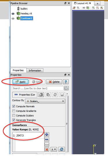
Figure 27: Value Range Selections
- If you do not see anything in the 3D window click the eye icon next to Contour1 in the Pipeline Browser
- This allows you to toggle between views in the 3D Viewer
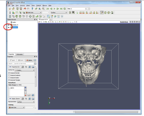
Figure 28: 3D Viewer
- Visually explore the dataset by looking at the visualization from all angles.
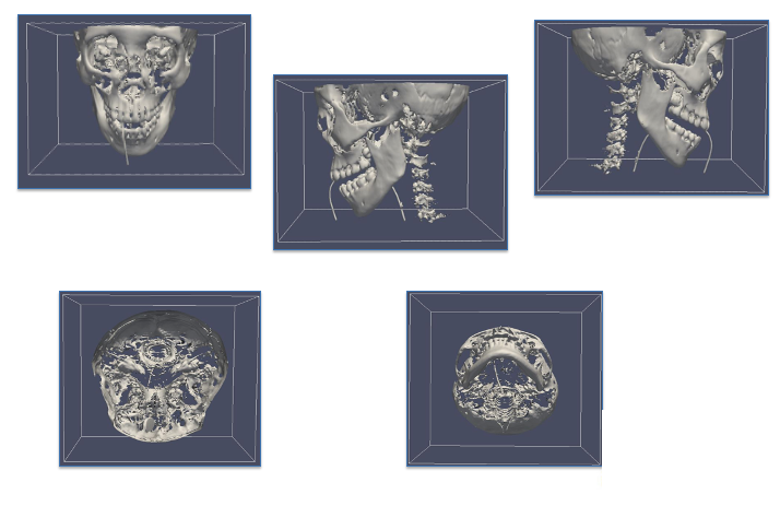
Figure 29: Visualization from different angles
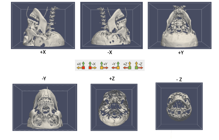
Figure 30: Visualization from different planes
The surface is often also called an isosurface.
Step 4:: Isosurfaces
You should be here:
Pipeline Browser:
1. Two Objects
2. Value Range [0, 4095]
- Select 2047.5 showing in Value Range. Selecting the value should highlight it.
- Delete that value (click the minus button to remove all values)
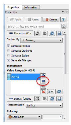
Figure 31: Delete Values
- Click the button below the minus button to: Add a Range Of Values
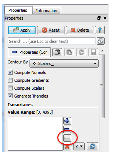
Figure 32: Range of Values
- Should see the Add Range Window
- Use this window to set the range of values
- For this tutorial
Min: 0
Max: 4095
- Feel free to pay around with the range (between 0 and 4905)
- Click OK
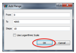
Figure 33: Range of Values
- Notice the Value Range: [0, 4095]
There are 10 values (steps) showing values between 0 and 4095
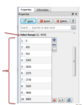
Figure 34: Range of Values Steps
- Apply the Contour
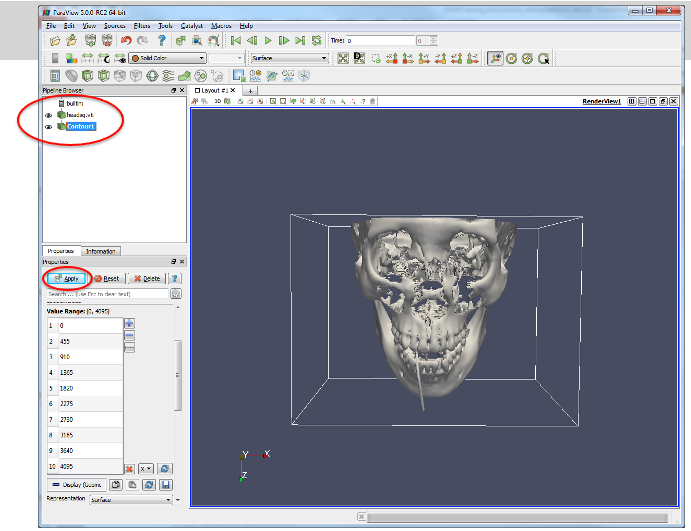
Figure 35: Contour
- This may take a few seconds to render.
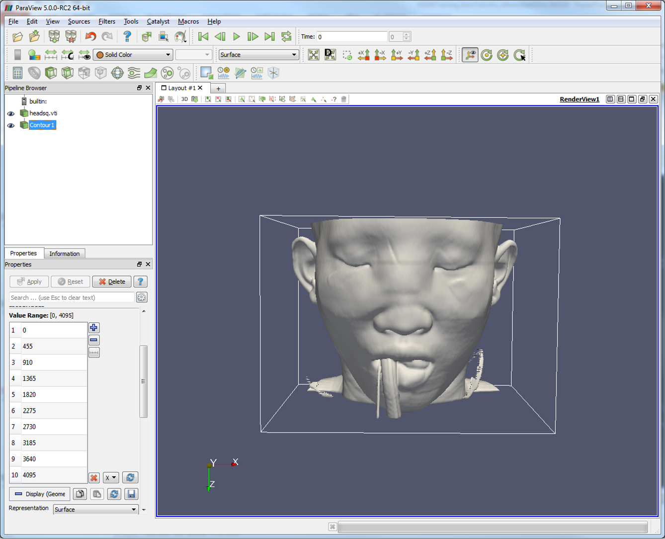
Figure 36: Rendered Visualization
- Explore the rendering.
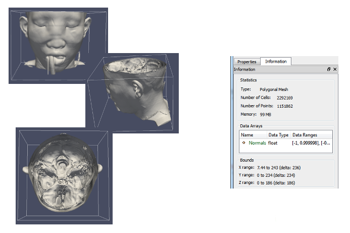
Figure 37: Explore Rendered Visualization
- Use this window to set the range of values
- For this tutorial
Min: 0
Max: 4095 - Feel free to pay around with the range (between 0 and 4905)
- Click OK
- Notice the Value Range: [0, 4095]
There are 10 values (steps) showing values between 0 and 4095
Step 5:: Explore the data set
Let's start working on varying the set value range
- Reset Vaues
- Click red X – Remove all entries.
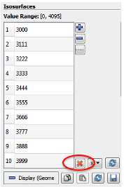
Figure 38: Remove entries
- Click Add a range of values button
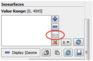
Figure 39: Add Range
- Click OK.
- Click Apply.
- You should be here:
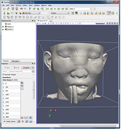
Figure 40: You should be here
- Clip Isosurface
- CLIP - Intersects the geometry with a half space.
The effect is to remove all the geometry on one side of a user-defined plane.
- Select Contour 1: (in pipeline Browser)
- Filters
- Common
- Clip
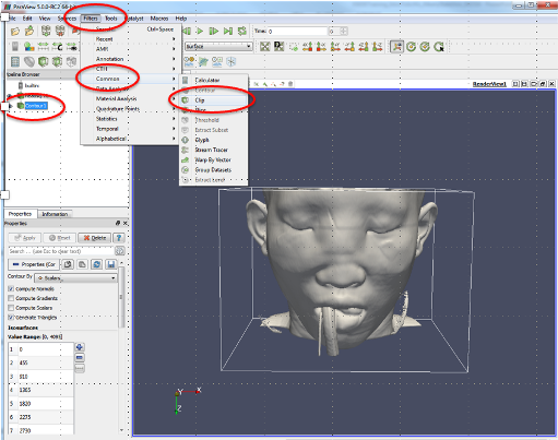
Figure 41: Clip
- A new object appeared in the pipeline browser (Clip 1).
- Clipping plane (see red vertical line and horizontal arrow)
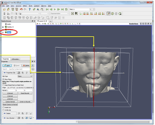
Figure 42: Clipping Pane
- Select the arrow point (arrow turns red)
- Rotate (drag) the arrow point until the arrow is pointing out of the screen toward you
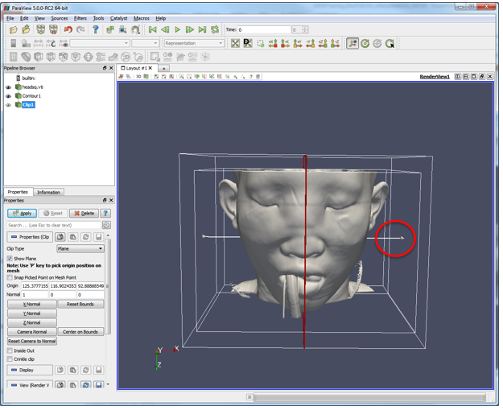
Figure 43: Arrow
- Resulting visualization.
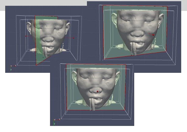
Figure 44: Resulting Visualization
- Click Apply after making your selection.
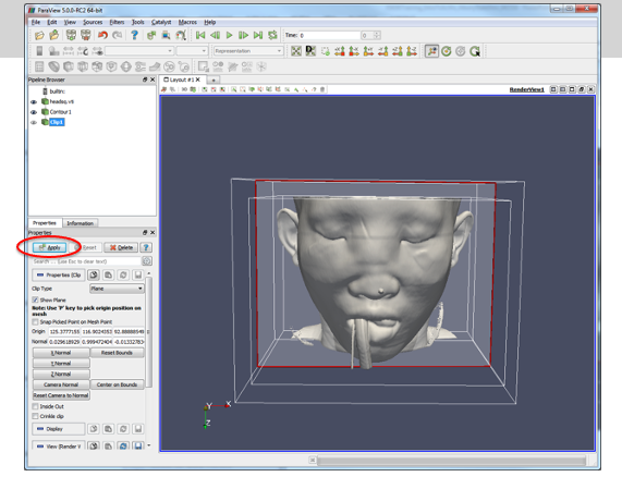
Figure 45: Apply
- Make sure the eye icon is not greyed out on the Clip1 object in the Pipeline Browser
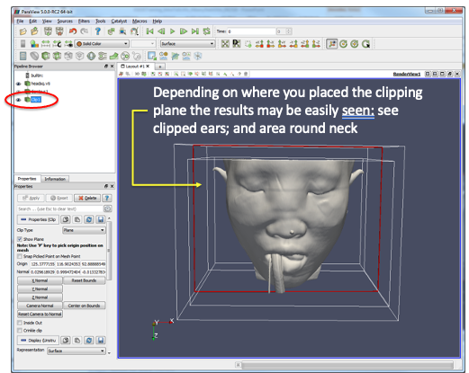
Figure 46: Eye
- Rotating the view reveals the clipped isosurface
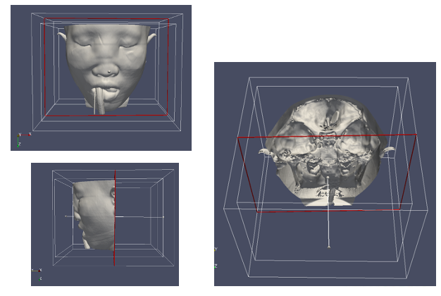
Figure 47: Rotated Views
- Click Apply after making your selection.
- Inside Out Property
If this property is set to 0, then clip filter will return that portion of the dataset that lies within the clip function.
If set to 1, the portions of the dataset that lie outside the clip function will be returned instead
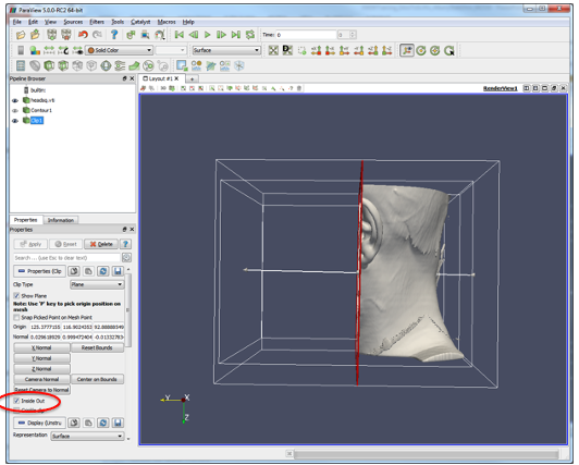
Figure 48: Inside Out Property
Slice Isosurface
- Click the eye icon next to Clip1 in the pipeline browser (hide the clip plot).
- Select Contour 1
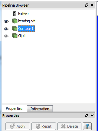
Figure 49: Eye
- Select Filters then Common and finally Slice.
On the map, click any state to view the pop-up. It should look like this:
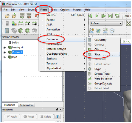
Figure 50: Filters
- Select Slice1.
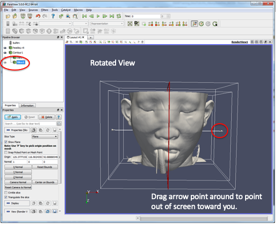
Figure 51: View
- Resulting Visualizations
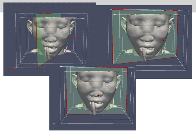
Figure 52: Resulting Visualizations
- Click Apply
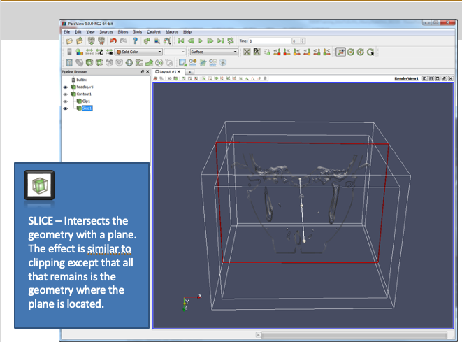
Figure 53: Summary
- Pipeline Browser
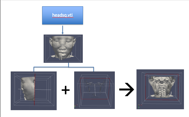
Figure 54: Pipeline Browser
- Click red X – Remove all entries.
- Click Add a range of values button
- Click OK.
- Click Apply.
- CLIP - Intersects the geometry with a half space.
The effect is to remove all the geometry on one side of a user-defined plane. - Select Contour 1: (in pipeline Browser)
- Filters
- Common
- Clip
- A new object appeared in the pipeline browser (Clip 1).
- Clipping plane (see red vertical line and horizontal arrow)
- Select the arrow point (arrow turns red)
- Rotate (drag) the arrow point until the arrow is pointing out of the screen toward you
- Resulting visualization.
- Click Apply after making your selection.
- Make sure the eye icon is not greyed out on the Clip1 object in the Pipeline Browser
- Rotating the view reveals the clipped isosurface
- Click Apply after making your selection.
If this property is set to 0, then clip filter will return that portion of the dataset that lies within the clip function.
If set to 1, the portions of the dataset that lie outside the clip function will be returned instead
- Click the eye icon next to Clip1 in the pipeline browser (hide the clip plot).
- Select Contour 1
- Select Filters then Common and finally Slice. On the map, click any state to view the pop-up. It should look like this:
- Select Slice1.
- Resulting Visualizations
- Click Apply
Step 6:: Saving your work.
There are many options to save your work:
- Save State
It saves the state of the visualization pipeline itself, including all the pipeline modules, views, their layout, and their properties.
This is referred to as the application state or, just, state.
In Paraview, you can save the state using the File Save State . . . menu option.
Conversely, to load a saved state file, you can use File Load State. . . . - Save Data
You can save the dataset produced by any pipeline module in ParaView, including sources, readers, and filters.
To save the dataset in paraview, begin by selecting the pipeline module in the Pipeline browser to make it the active source.
For modules with multiple output ports, select the output port producing the dataset of interest.
To save the dataset, use the File Save Data menu or the button in the Main Controls toolbar. You can also use the keyboard shortcut Ctrl + S (or + S ).
The Save File dialog will allow you to select the filename and the file format. The available list of file formats depends on the type of the dataset you are trying to save. - Save Screenshot
To save the render image from a view in paraview, use the File Save Screenshot menu option. This will pop up the Save Screenshot Options dialog.
This dialog allows you to select various image parameters, such as image resolution and image quality (which depends on the file format chosen).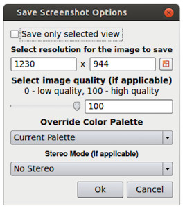
Figure 56: Screenshot Dialog
By default, Paraview will save rendered results from the active view. Optionally, you can save an image comprising of all the views layed out exactly as on the screen by unchecking the Save only selected view button.
Conclusion
After following this tutorial you should be able to get started with creating custom scientific visualizations using Paraview.
here are some additional resources to help you learn more about using Paraview:
- ParaView Documentation: The official ParaView documentation is an excellent resource for understanding the software's features, workflows, and capabilities. It provides detailed explanations, tutorials,
and examples to help users get started and explore advanced topics. You can find the documentation at: https://docs.paraview.org/
- ParaView Tutorial Videos: The ParaView website offers a collection of tutorial videos covering various aspects of using ParaView for scientific visualization. These videos provide step-by-step instructions
and demonstrations, making it easier to grasp the software's functionality. You can access the tutorial videos at: https://www.paraview.org/tutorial/
- ParaView Guide: "The ParaView Guide" is a comprehensive book written by the creators of ParaView. It provides in-depth coverage of ParaView's features, including data processing, visualization techniques,
and advanced topics. The guide offers practical examples and insights into effective scientific visualization practices. You can find the book on the ParaView website or online booksellers.
- Online Courses and Webinars: Several online platforms and institutions offer courses and webinars specifically designed to teach ParaView. These resources provide structured learning experiences, often
with hands-on exercises, to help users gain proficiency in using the software. Platforms like Coursera, Udemy, and edX may have relevant courses available.
- Example Data and Tutorials: ParaView provides a collection of example datasets and tutorials that cover various scientific visualization scenarios. These resources can be accessed within the software
itself and offer practical hands-on experience to learn specific visualization techniques and workflows.
ParaView and Python Shell
We will be going through the steps to utlize the Python Shell for scripting in Paraview.
Step 0: Setting up the Python Shell
- Click on Edit in the toolbar and select Reset Session.
- Setting up the Python Shell
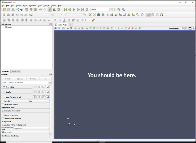
Figure 1: User Interface
- Click on View in the toolbar and check the Python Shell.
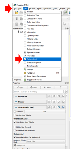
Figure 2: View Options
- Interface
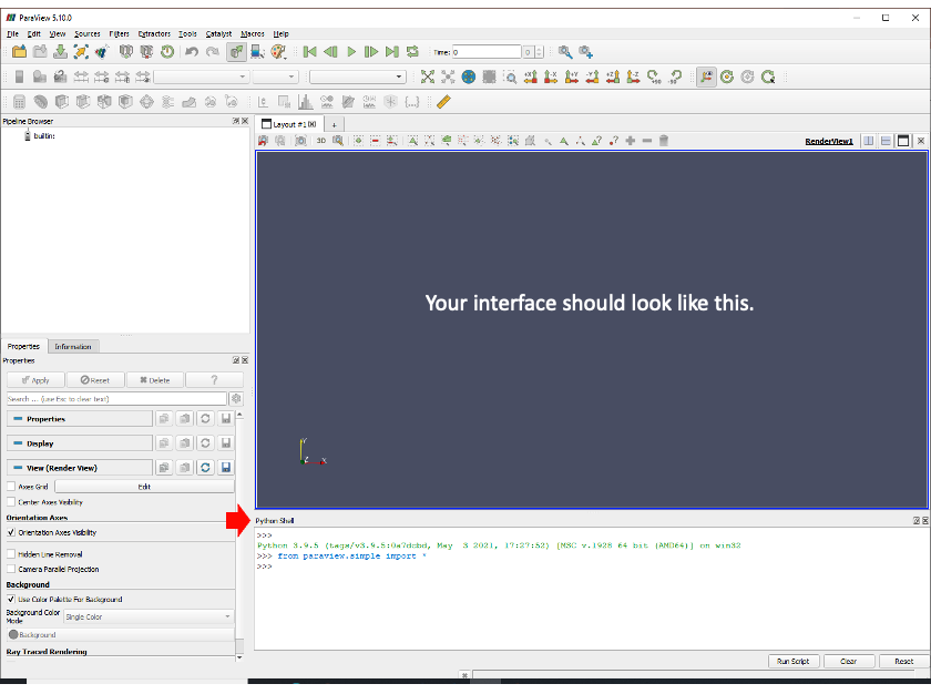
Figure 3: Shell visible in interface
- About ParaView and Python Shell
- You can copy commands from elsewhere and paste them into the Python Shell
- Python is case sensitive. Be sure to use the correct capitalization as shown.
- Python is indent sensitive. Be sure to not indent.
- Saving your output
- Save a Screenshot
- Must show render window and python scripting window
- Save as PythonScritping output
LastnameFirstInitial_ParaViewPythonFig#.jpg
- You can copy commands from elsewhere and paste them into the Python Shell
- Python is case sensitive. Be sure to use the correct capitalization as shown.
- Python is indent sensitive. Be sure to not indent.
- Save a Screenshot
- Must show render window and python scripting window
- Save as PythonScritping output
LastnameFirstInitial_ParaViewPythonFig#.jpg
Step 1: Creating a Pipeline
- Type the following into the Python Shell.
>>> sphere = Sphere()
>>> Show()
>>> Render()
>>> ResetCamera()
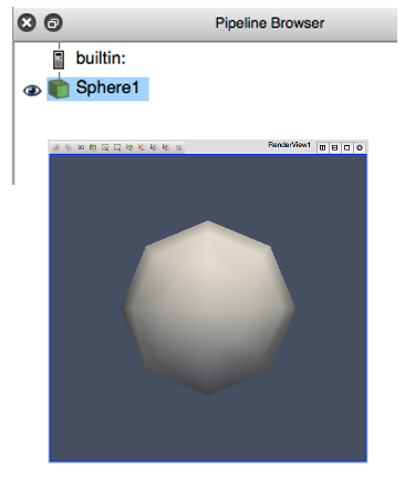
Figure 4: Sphere
- In Python Shell create a source
>>> sphere = Sphere()
>>> Show()
>>> Render()
>>> ResetCamera()
- Then feed that into a filter
>>> Hide()
>>> shrink = Shrink()
>>> Show()
>>> Render()
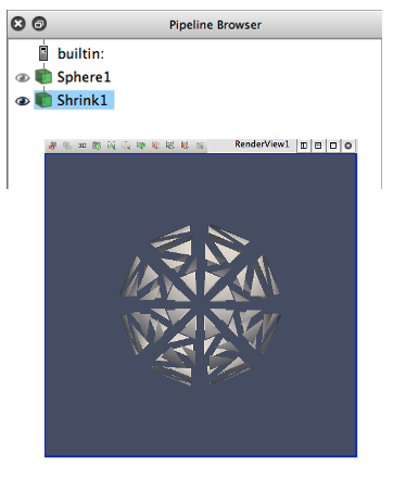
Figure 5: Sphere with filter
>>> sphere = Sphere()
>>> Show()
>>> Render()
>>> ResetCamera()
>>> sphere = Sphere()
>>> Show()
>>> Render()
>>> ResetCamera()
>>> Hide()
>>> shrink = Shrink()
>>> Show()
>>> Render()
Step 2: Changing Properties
- Get listing of sphere’s properties
>>> dir(sphere)
- Examine and then change one
>>> print(sphere.ThetaResolution)
>>> sphere.ThetaResolution=16
>>> Render()
- Change a different filter
>>> shrink.ShrinkFactor = 0.25
>>> Render()
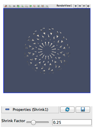
Figure 6: Sphere with different properties
>>> dir(sphere)
>>> print(sphere.ThetaResolution)
>>> sphere.ThetaResolution=16
>>> Render()
>>> shrink.ShrinkFactor = 0.25
>>> Render()
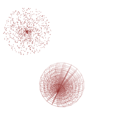
Step 3: Branching and Merging Pipelines
- Feed sphere’s output into a second filter
>>> wireframe = ExtractEdges(Input=sphere)
>>> Show()
>>> Render()
- Feed two filters into one
>>> group = GroupDatasets(Input=[shrink,wireframe])
>>> Show()
>>> Hide(shrink)
>>> Hide(wireframe)
>>> Render()
- Change a different filter
>>> shrink.ShrinkFactor = 0.25
>>> Render()
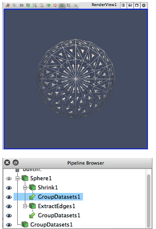
Figure 7: Group Datasets
>>> wireframe = ExtractEdges(Input=sphere)
>>> Show()
>>> Render()
>>> group = GroupDatasets(Input=[shrink,wireframe])
>>> Show()
>>> Hide(shrink)
>>> Hide(wireframe)
>>> Render()
>>> shrink.ShrinkFactor = 0.25
>>> Render()
Finding Pipeline Objects
- GetSources() - Returns a list of objects listed in the Pipeline Browser
- GetActiveSource() - Returns the object selected in the Pipeline Browser
- SetActiveSource() - Sets the object selected in the Pipeline Browser to the given object
Exercise
- Create a new pipeline
>>> cone = Cone()
>>> help(cone)
- This gives you the full list of properties. What is the resolution?
>>> cone.Resolution
- Increase the resolution to 32.
- What is the cone’s center? Change the center to 1, 2, 3.
>>> cone.Center=[1,2,3]
- Apply a shrink filter to the cone.
>>> shrinkFilter = Shrink(cone)
>>> shrinkFilter.Input
- Create a Cone Object
>>> shrinkFilter.UpdatePipeline()
>>> shrinkFilter.GetDataInformation().GetNumberOfCells()
>>> shrinkFilter.GetDataInformation().GetNumberOfPoints()
- What we did:
- Create Cone Object
- Set Cone Resolution
- Set Cone Center Properties
- Apply Shrink Filter to the Cone
- Update Pipeline
- Rendering
Two objects are needed to render the output
- A representation – takes a data object and renders it in a view
- A view – is responsible for managing a render context and a collection of representations
- Rendering the Object
>>> Show(shrinkFilter)
>>> Render()
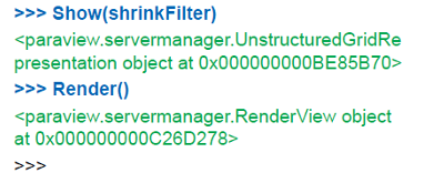
Figure 8: Rendering Shell Output
>>> cone = Cone()
>>> help(cone)
>>> cone.Resolution
>>> cone.Center=[1,2,3]
>>> shrinkFilter = Shrink(cone)
>>> shrinkFilter.Input
>>> shrinkFilter.UpdatePipeline()
>>> shrinkFilter.GetDataInformation().GetNumberOfCells()
>>> shrinkFilter.GetDataInformation().GetNumberOfPoints()
- Create Cone Object
- Set Cone Resolution
- Set Cone Center Properties
- Apply Shrink Filter to the Cone
- Update Pipeline
Two objects are needed to render the output
- A representation – takes a data object and renders it in a view
- A view – is responsible for managing a render context and a collection of representations
- Rendering the Object
>>> Show(shrinkFilter)
>>> Render()
Review
Horizonal assessment of GIS core concepts mapped to Bloom’s Taxonomy of Hierarchical Learning
What you should know:
| Bloom’s Taxonomy Hierarchy | You should know |
|---|---|
| Remember | Recall basic GIS concepts. |
| Understand | Define basic GIS concepts. |
| Apply | Use symbolization, classification, and data skills to make a new map for different regions. |
| Evaluate | Consider ethical and communications implications of your chose of variables, colors and map projects in in your final visualizations |
| Analysis | Compare and contrast different physical or cultural regions, question the difference that imagery at a different scale would make on your assessment of land and use change |
| Create | Design, create, and give a presentation using multimedia web-GIS maps and web mapping applications. |
Resources
Download ParaViewEffective Mapping in Tableau
What you should be able to do:
| You should be able to do | |
|---|---|
| Factual | Understand terms such as plate, continent, ocean, fault line, depth, magnitude and others. |
| Conceptual | Understand how different variables affect overall quality of geographic content |
| Procedural | Demonstrate how to perform specific tasks in a geographic information system (GIS) , collect data, and map results. |
| Metacognitive | Apply strategic knowledge about to approach a problem using GIS, spatial data, and the spatial perspective. |